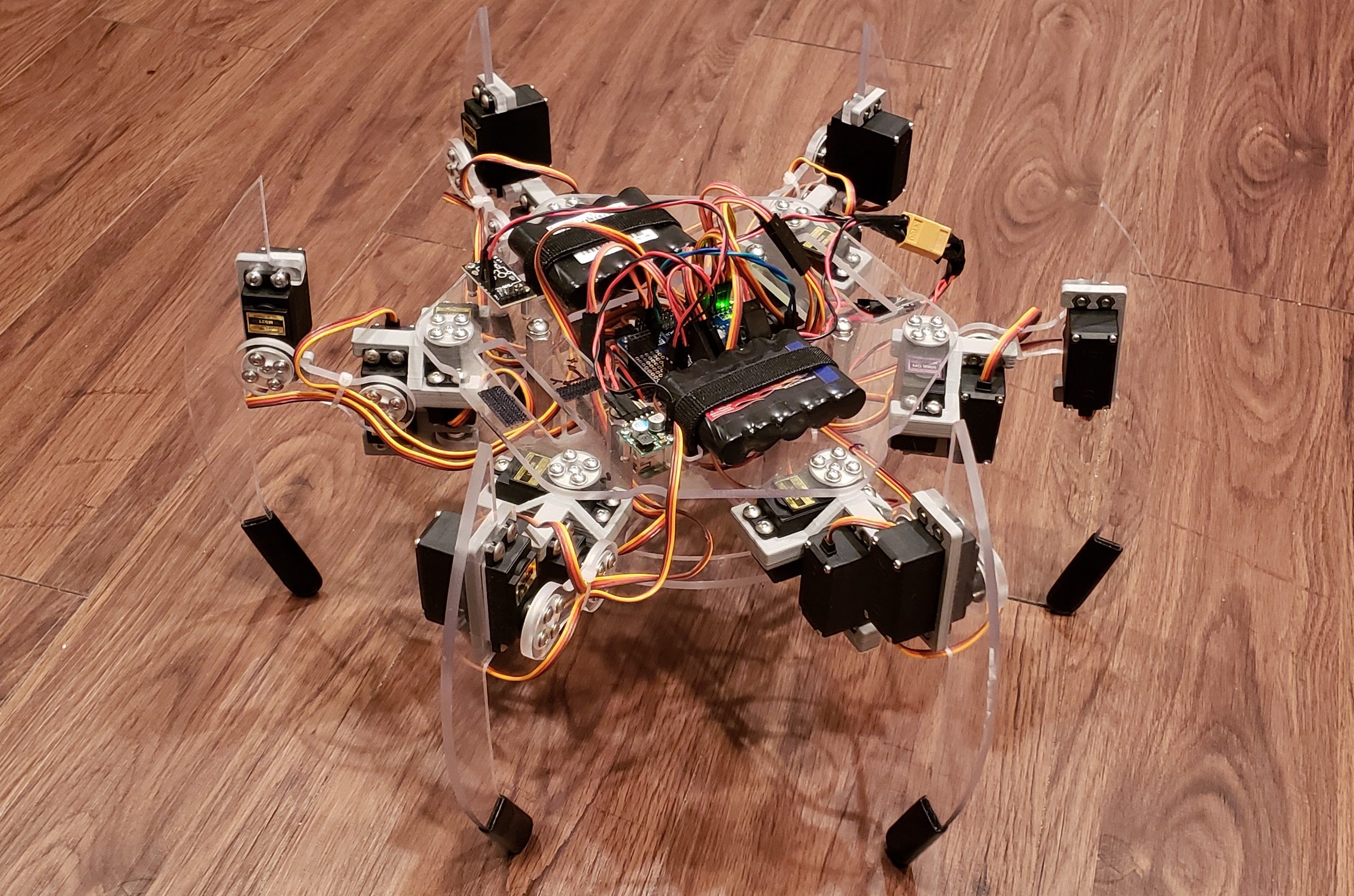
I’ve always wanted to build a hexapod. It seems like such a classic “maker” project but I was always intimidated by the controls that are involved. After all, 6 legs means 18 servos and that means programming the control system can get really messy really fast. However, thanks to some recent coursework at my university, I finally felt confident enough to tackle this project!
There is a lot to cover here so take a look at the table of contents below to see how everything is organized. All of the published Python and MATLAB code, as well as the CAD files, are available for download at the bottom of this page.
Mechanical Design
I started the project by designing a leg with three degrees of freedom in Solidworks with a couple of spare MG996R servos I had on hand. At this early stage, I had the following design constraints:
- Be easy to fabricate with my available tools (3D printer or CNC router).
- Links between servos should be as stiff as possible.
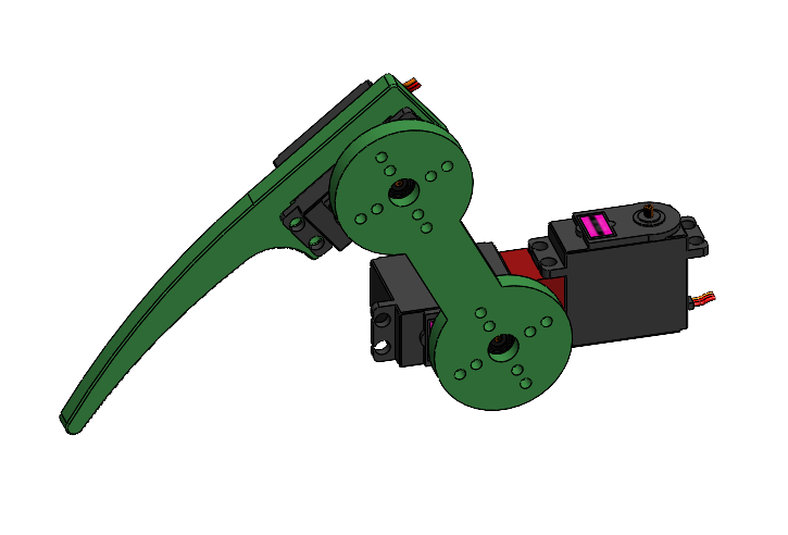
An early leg design. 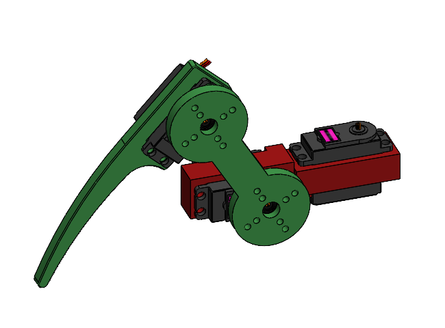
A later leg design.
The biggest challenge was designing the “knuckle” that connects the first servo to the second servo (shown in red on the above figures). The geometry was complex compared to the rest of the leg. Furthermore, the secondary shear force (that which is experienced out of phase with the output shaft) would cause a non-negligible moment because of the distance between the two output shafts. Consequently, the part would experience a larger internal stress.
Using my 3D printer and an Arduino, I was able to produce some “proof of concept” legs very quickly.
Considering the aforementioned stress analysis of the knuckle, and by sketching out a rough free-body-diagram of each leg, three more design constraints were added.
- Distance between the output shafts of the first and second servo (L1) should be minimized.
- Distance between the first servo and the center of the robot (LF) should be minimized.
- The entire weight of the robot should be supported by at least 5 legs (at least 1 leg needs to be in the air to walk).
The distance from the second servo to the third servo (L2), and the distance from the third servo to the end effector (L3) was also considered for the torque analysis. However, those values also play a critical role in the kinematic study. I’ll go into more detail about how I determined those lengths in the “MATLAB Simulation” section of this post.
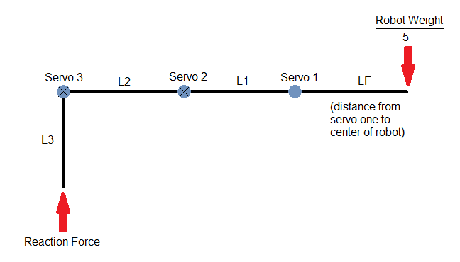
The rated torque of the MG996R is 11 kg∙cm. By balancing moments about each servo, we can determine whether the torque experienced by each servo exceeds the rated torque. When using the estimated weight of the robot (found in Solidworks) and the chosen leg lengths, the torque experienced by servos 2 and 3 in the critical configuration is about 9 kg∙cm.
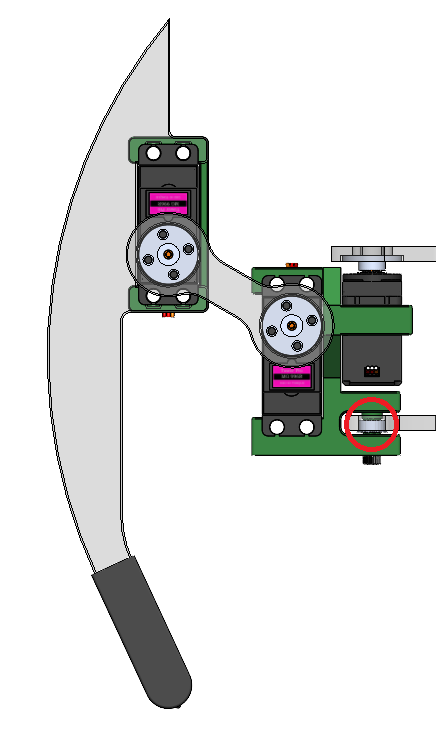
The final version of the leg includes a bearing on the first servo to absorb the cantilever load which is applied perpendicular to the output shaft of the first servo (highlighted in red above).

Fabrication and Assembly
All of the parts were either 3D printed out of PLA or milled out of 3/16″ acrylic on a CNC router. The following pictures show the 3D printed knuckle and its sub-assembly with the servos installed.
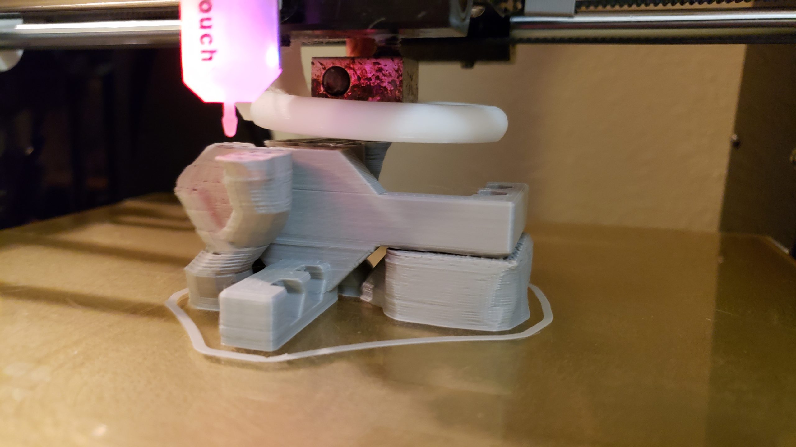
Printing a knuckle. 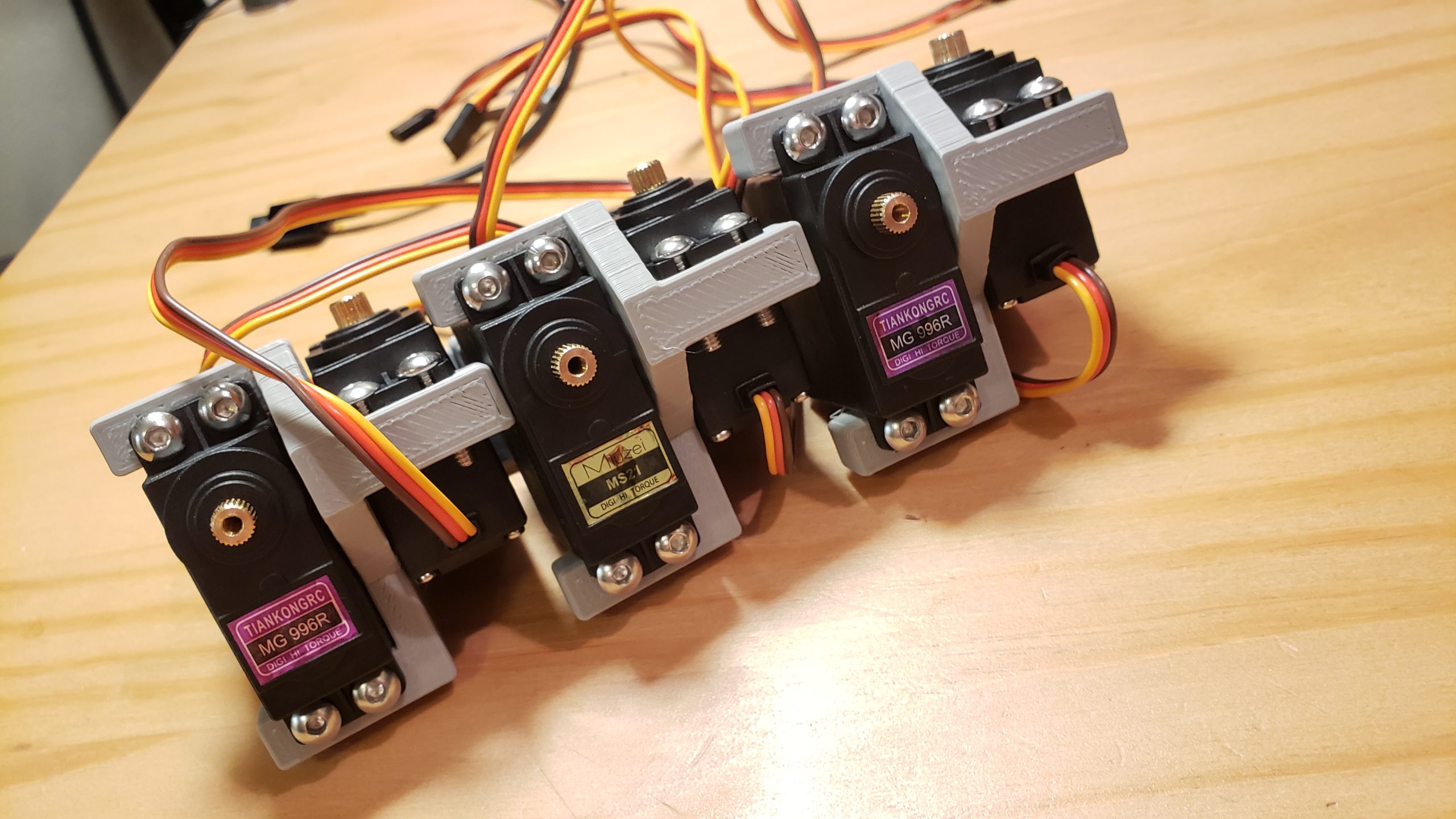
Multiple assembled knuckles. 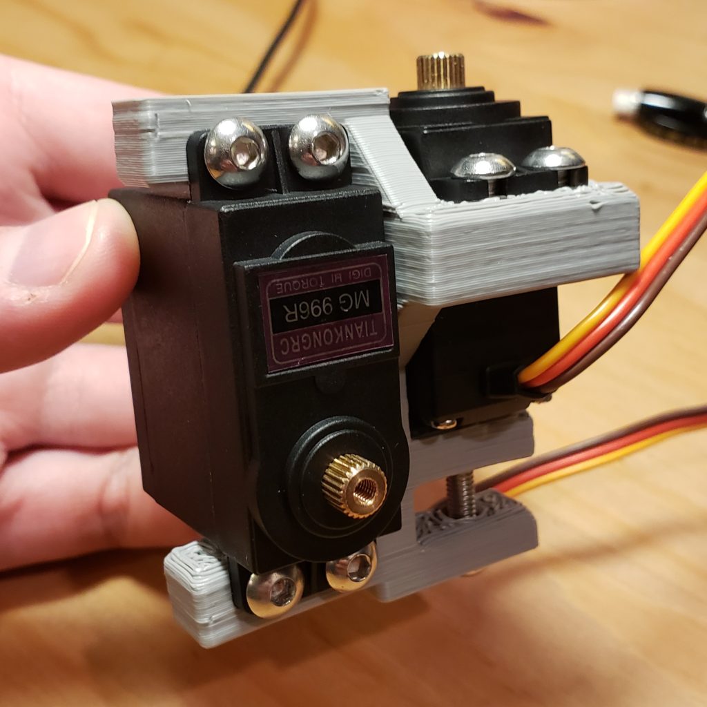
Single assembled knuckle.
The following photos show the milled parts. I had a bunch of 3/16″ acrylic left over from building an enclosure for the Shapeoko 3 so I used that. I was skeptical about the flex in the acrylic but it didn’t turn out to be a problem.
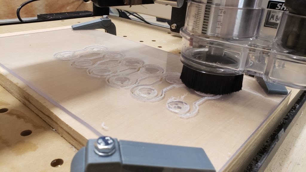
Cutting several mid-arms. 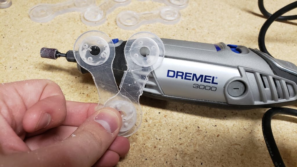
Processing mid-arms. 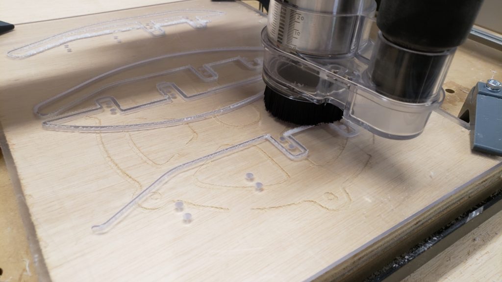
Cutting several forearms. 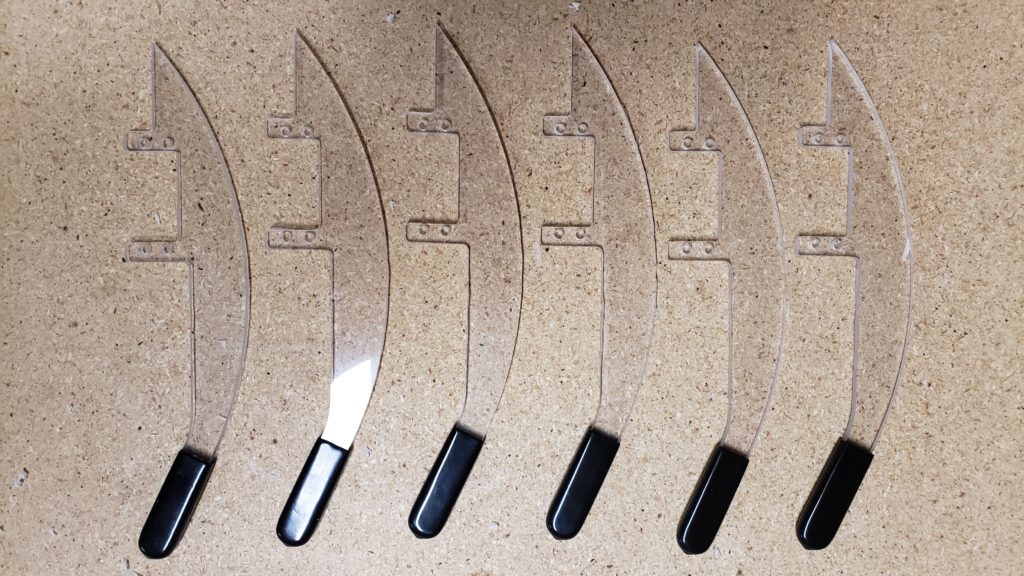
Several completed forearms.
Everything came together really well. I was extremely pleased with how well the parts fit together. The only play in the legs is coming from run-out at the output shaft of the servos; not flex in the acrylic.
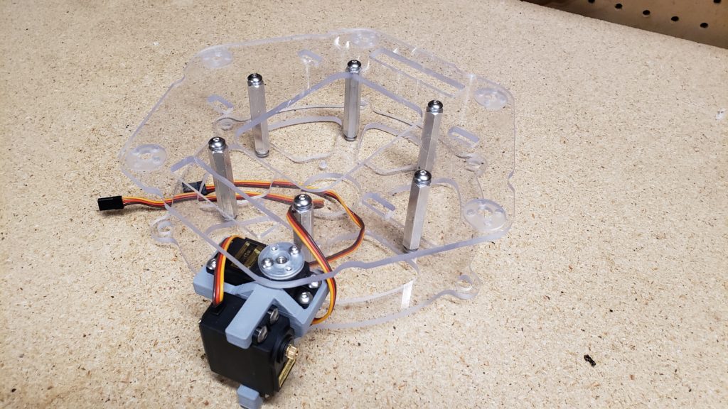
Partially assembled frame. 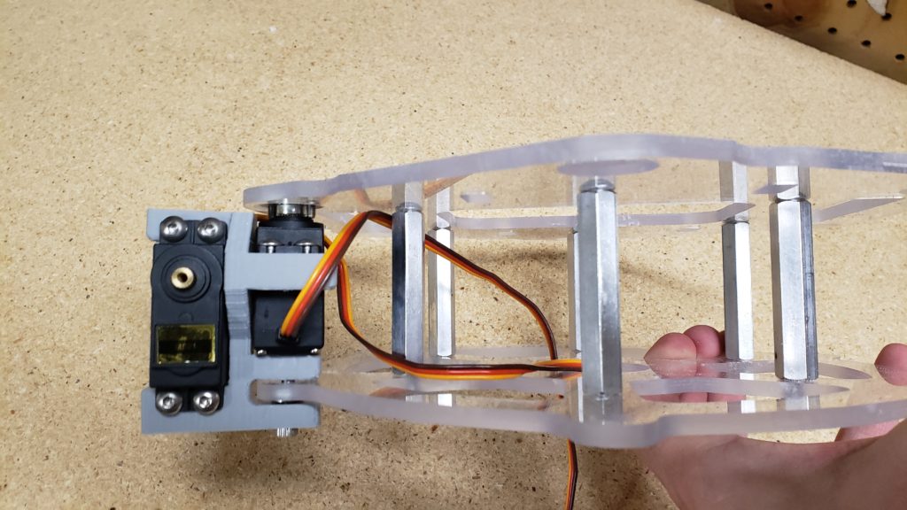
Partially assembled frame. 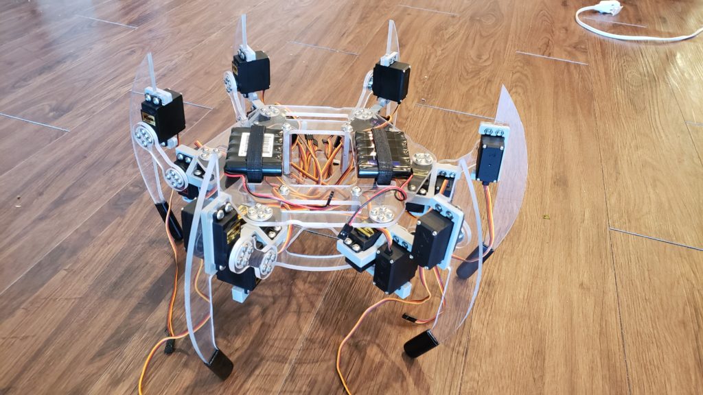
Assembled hexapod without controller.
Now I have a tin man. Time to get to work adding a brain!
MATLAB Simulation
To control the robot, I could send individual angle commands to the servos. However, because we have 3 servos per leg, this would be really tedious to implement. Especially because some of the operations I want to perform involve holding one of the coordinates of the foot constant while changing the other coordinates (e.g. A walking motion involves keeping the “height” of the foot constant as it moves across the ground). Instead, I’ll develop a solution that gives me the unknown joint angles for a desired foot location in Cartesian space (end-effector).
Why use MATLAB? Two big reasons:
- It’s easy to burn out a servo if it’s directed to go to a location that it can’t actually reach (e.g. commanded to rotate 95° but it can only go 80° before it runs into something that it isn’t strong enough to move). MATLAB acts as a “safe” place to test code before going to physical hardware.
- I need to validate the algorithms I’m creating in an “ideal” space. Because these are cheap servos, there will be some position error even with perfect code. With MATLAB I’ll be able to differentiate between “code problems” and “hardware problems” when troubleshooting.
So, first I’m going to develop an algorithm in MATLAB that will plot the orientation of the leg for a given set of joint angles and leg lengths (forward kinematics). After that, I’ll work that algorithm backwards to get the unknown joint angles for a known Cartesian coordinate (inverse kinematics).
Forward Kinematics
Let’s start by defining some kinematic terms:
- Theta: The joint angle of a servo. The joint is always oriented in the Z-axis.
- Delta: The distance offset to the next joint in the direction of the output shaft.
- a: The distance offset to the next joint in the direction of the common normal. The common normal is always oriented towards the X-axis.
- Alpha: The amount of rotation about the previous common normal in order to make the current joint parallel to the next.
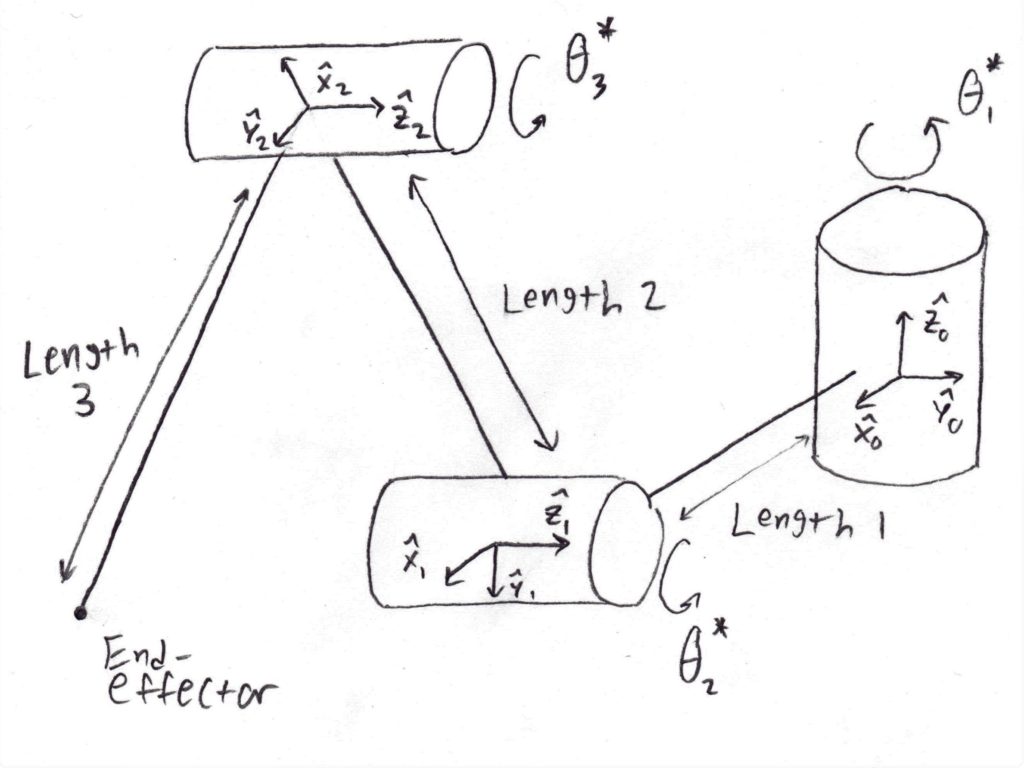
Below, is a Denavit-Hartenberg (DH) table for the parameters previously discussed.
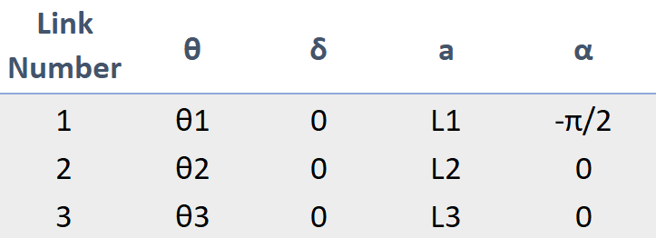
By treating every cell in the DH table as a homogenous-transformation matrix, and by then multiplying all of the rows of the table together, we can determine the end-effector location for any desired joint angle.
With a little bit of linear algebra and a couple of trigonometric identities, we can arrive at the following solution for the end-effector coordinates (xf, yf, zz) given a known set of joint angles and link lengths:
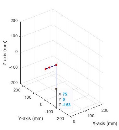
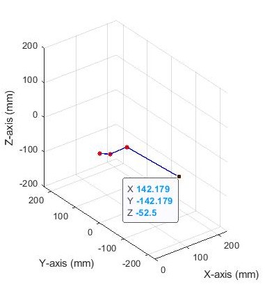
Plugging these values into MATLAB and plotting the results can quickly reveal what different joint angles look like. The figure on the left shows the leg with joint angles of 0°, 0°, and 90°. The figure on the right shows the leg with joint angles of -45°, -30°, and 60°.
We can use a loop to iterate through all the possible joint angles. This is very useful for determining all the “kinematically possible” locations of the end effector.
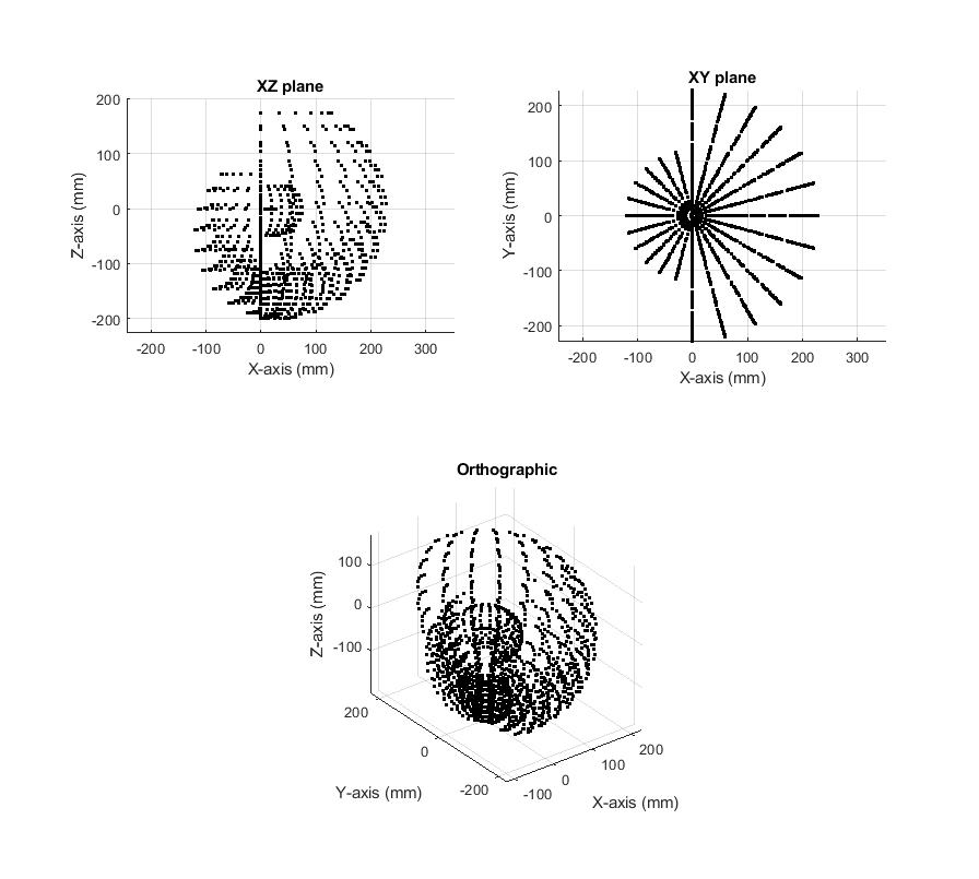
The MATLAB code that was used to produce all of these plots is available at the bottom of this post.
Inverse Kinematics
Now that we have an understanding of how to get the end-effector location from the link lengths and joint angles, let’s work that backwards. That is, let’s determine the required joint angles for a desired end-effector location (we’ll assume that link lengths are known).
We’ll start with one of the intermediate equations from the forward kinematics derivation and use some linear algebra to move things around:
In real-world terms, by moving the transformation matrix for the first joint angle to the left side of the equation, I have actuated the second and third joint before the first. All that is left to do is actuate the first to solve the equation. It follows, then, that the z-coordinate of the end effector will not be affected by this last change (a rotation about the z-axis doesn’t change the z-values of a point in space). Furthermore, the x and y coordinates will only change across a circular path. This observation is referred to as “invariance” and is described mathematically as follows.
Note: The trigonometric addition identity was used to simplify the equations; cos(ϴ23) = cos(ϴ2+ϴ3)
Using the invariance equations, we can rearrange and eliminate terms using trigonometric identities to solve for the joint angles.
The equation for the third joint angle is now known. We can use that to solve for the other joint angles. This time, we’ll take the invariance equations and put it into matrix form.
We can take the inverse of the matrix with the ϴ3 terms to isolate the ϴ2 terms.
The equation for the second joint is now known. Lastly, we can derive joint one simply by observing that links 2 and 3 are co-planar. As a result, joint one is only a function of the x-coordinate and the y-coordinate.
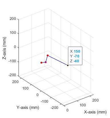
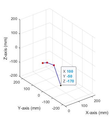
These equations will drive the servo angles for the hexapod. The figure on the left shows a commanded coordinate of 150mm, -70mm, and -40mm (X,Y,Z). The figure on the right shows a commanded coordinate of 100mm, -50mm, and -170mm (X,Y,Z).
Trajectory Planning
To make the leg walk, let’s consider a set of coordinates that we want the leg to periodically cycle through. The figure below shows a set of coordinates that will produce locomotion towards the positive Y-axis.
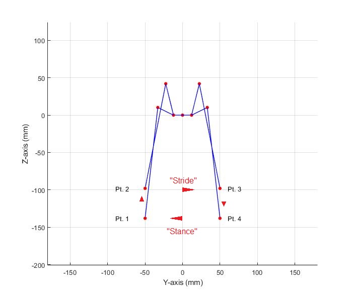
We can divide this trajectory into two phases: a “stride” and a “stance.” The stride phase is when the leg is in the air. The stance operation is when the leg is pushing across the ground.
The stance phase should always be constant velocity. Any variation of velocity between the end-effectors as they push on the ground could cause the servos to fight each other. To achieve this, we’ll use linear interpolation:
For the stride operations, we just want the leg to get to the next point as quickly as possible without overshooting the target or damaging the servo. To achieve this we’ll use sinusoidal interpolation:
Sinusoidal interpolation is great for this application because the velocity and acceleration of the end-effector is guaranteed to be zero at the start and end of time (derivatives at t=0 and t=tf are zero).
Lastly, we’ll create a piece-wise function which contains four interpolations. Our tunable variables will be tstance, the time it takes to perform the stance operation, tstride, the time it takes to perform the stride operation, and tperiod, the summation of the time required for all the operations.
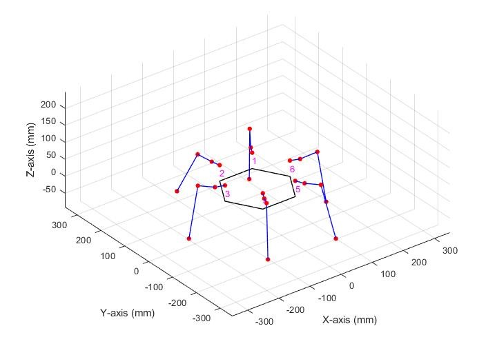
In order to sequence each leg in the set, we add a certain fraction of tperiod to each leg’s current time. This “time vector” produces different walking gaits depending on the fractions selected. For instance, here is the vector for moving one leg in the air at a time:
If we want to move two legs in the air at a time:
If we want to move three legs in the air at a time:
Note: It is possible to move with four legs in the air at a time (a “galloping” gait). However, this would require dynamic control which can adjust the robot’s balance. This is something I would like to work on in the future.
Testing
After converting all of the MATLAB formulas to Python code, we’re ready to take the first steps! The following video shows Brigg’s executing three simple commands:
- Stand up.
- Walk with two legs in the air in a direction 60° from the X-axis for 400mm.
- Sit down.
This next video shows Briggs walking with one leg in the air at a time.
The next video shows Briggs walking with three legs in the air at a time.
Conclusions and Future Plans
I’m really happy with how the build of Briggs came out. However, the run-out in the servos gets on my nerves sometimes. This could be solved by either (A) buying better servos or (B) designing a bearing support for the second and third joint like the first joint has. Of course, the extra weight would be too much for these cheap servos to handle. So the long term solution is better servos. The good news is there are vastly stronger, higher quality servo options online (albeit at a vastly steeper price) that fit the same form factor as the current servos (no redesign needed!)
The Python code needs to be cleaned up a lot. Juggling the classes I made for these six legs was a learning experience for me. Some of my implementation just won’t scale well. For instance, (besides the gait function) each leg currently gets its own loop for striding. This means that two or more legs can’t stride simultaneously…
I have a laundry list of things I would like to experiment with so I should be busy for awhile:
- Teleoperated control
- Software correction for veering (e.g. “robot is pulling to the right/left”)
- Implementing line following with OpenCV and a webcam
- Frame orientation inverse kinematics
- Dynamically corrected frame orientation with an IMU
Bill of Materials
| Item | Cost | # of Units | Total |
|---|---|---|---|
| Raspberry Pi 3 B+ | $35 | 1 | $35 |
| Adafruit Servo-Hat | $16 | 2 | $32 |
| 5V 2.5Amp Voltage Regulator | $9 | 1 | $9 |
| 6V 2000mAh NiMH Battery | $12 | 2 | $24 |
| MG996R Servo | ~$4.5 | 18 | $81 |
| Aluminum Servo Horn | $1 | 18 | $18 |
| F684ZZ Flanged Bearing | $1 | 6 | $6 |
| Grand Total: | $205 |
Links to code and CAD
Python repository: https://github.com/Lazerkill/Briggs/tree/main/Python
Note: Python code requires Adafruit Servo Hat libraries to be installed first.
MATLAB repository: https://github.com/Lazerkill/Briggs/tree/main/Matlab
Solidworks repository: https://grabcad.com/library/briggs-the-hexapod-1

